
To create a drop-down list in Microsoft Excel, select the cells, go to Data > Data Validation, choose List under Allow, and type your options separated by commas or select a range of cells. Click OK, and each cell shows an arrow when you select it. You can change or remove the list in the same dialog.
Drop-down lists help keep spreadsheet entries consistent by letting you choose from predefined options instead of typing them manually. They're useful for tracking project statuses, assigning tasks, recording customer information, and organizing other data with repeated values. This guide covers how to create a drop-down list, edit its options, remove it without losing your data, and make one list depend on another.
How to create a drop-down list in Excel
You create a drop-down list in Excel by adding a Data Validation rule of the List type to the cells you choose. The whole setup happens in one dialog box. Take a Status column in a 200-row task tracker as an example:
1. Select the cells that should get the list, for example B2:B200.
2. Go to the Data tab and click Data Validation.
3. Open the Settings tab.
4. Choose List in the Allow box.
5. Fill in the Source box: type the entries separated by commas (Open,In progress,Done), or click in the box and select the cells that hold the list.
6. Keep In-cell dropdown selected. Leave Ignore blank selected if empty cells are allowed.
7. Click OK.
8. Select one of the cells and click the arrow to test the list.
Two optional tabs sit next to Settings. Input Message shows a hint when someone selects the cell. Error Alert decides what happens when someone types a value that is not on the list.
Tip: keep long lists on a separate sheet. Put the entries on their own sheet (call it Lists) and point the Source box at that range. The list stays out of the way, and you edit it in one place instead of inside a dialog box. Microsoft recommends formatting the source as an Excel Table: select a cell in it and press Ctrl+T.
On a long tracker, freezing the header row keeps the column names in view while you fill in the list cells further down.
Want to try the same task in an alternative office suite? MobiSheets adds a dropdown list straight from its Insert menu.
Where the list entries should come from
Excel drop-down lists can use manually typed entries, a cell range, or a source that updates as your data grows. The right option depends on how often you'll need to change the available choices.
For short, fixed lists, typing the entries directly is usually the quickest option. For longer lists, referencing cells makes future changes easier.
Before creating your list, consider removing duplicate entries from the source data so the same option doesn't appear more than once.
How to edit a drop-down list
To edit a drop-down list in Excel, open Data Validation and update its Source field. The process depends on whether you originally typed the options or selected them from a cell range.
If you typed the entries manually:
1. Select a cell containing the drop-down list.
2. Go to Data > Data Validation.
3. Open the Settings tab.
4. Edit the values in the Source field, keeping them separated by commas.
5. Click OK to save your changes.
For example, you can change Pending,Approved,Rejected to Pending,Under Review,Approved,Rejected without creating a new list.
If your list uses a cell range:
1. Find the cells containing the original options.
2. Edit, replace, or remove the values directly in those cells.
3. If you've added entries outside the original range, open Data Validation and update Source to include them.
4. Click OK.
If the same validation settings are used across multiple cells, select Apply these changes to all other cells with the same settings in the Data Validation dialog.
This updates the matching drop-down lists together instead of requiring you to edit each one individually.
For lists that change regularly, an Excel Table can reduce maintenance because newly added rows can become part of the list source.
How to remove a drop-down list
You can remove a drop-down list in Excel without deleting the values already selected in its cells. Simply clear the Data Validation rule rather than deleting the cell contents.
Follow these steps:
1. Select the cell or range containing the drop-down list.
2. Go to Data > Data Validation.
3. Open the Settings tab.
4. Click Clear All.
5. Click OK to confirm.
The drop-down arrow disappears, but existing cell values remain unchanged. You can then type new entries into those cells without being limited to the previous list.
This is useful when a spreadsheet no longer needs restricted entries but you want to preserve the information already recorded.
How to make a dependent drop-down list
A dependent drop-down list changes its available options based on the value selected in another cell. For example, choosing a country in the first list can determine which cities appear in the second.
You can build this using named ranges and the INDIRECT function.
Example: Country and City drop-down lists
Suppose you're creating a spreadsheet where users first select a country and then a city.
Step 1: Prepare your source data.
Create two columns with the city options:
Step 2: Name each range.
Select the Bulgarian cities without the header and enter Bulgaria in the Name Box. Repeat for the French cities, naming the range France.
The range names must match the options in your first drop-down list.
Step 3: Create the country drop-down list.
Select cell A2 and go to Data > Data Validation.
Under Allow, choose List and enter the following in Source:
Bulgaria,France
Click OK.
Step 4: Create the dependent city list.
Select cell B2 and open Data Validation again.
Choose List and enter this formula in Source:
=INDIRECT(A2)
Click OK.
Now, when you choose Bulgaria in A2, the list in B2 contains Sofia, Plovdiv, and Varna. Changing A2 to France makes the city list offer Paris, Lyon, and Marseille.
The INDIRECT function converts the text in A2 into a reference to the corresponding named range.
This method is useful for product categories, departments, locations, and other related data. You can also use spreadsheet formulas and functions to work with values selected from lists.
Note: Changing the first selection updates the second list's available options, but it does not automatically clear a previously selected value in the second cell.
Drop-down list problems and how to fix them
Most Excel drop-down list problems come from incorrect Data Validation settings or a source range that no longer matches your data. Here are four common issues and how to resolve them.
The drop-down arrow doesn't appear. Excel normally shows the arrow only when the cell containing the list is selected. If it's still missing, open Data > Data Validation > Settings and make sure In-cell dropdown is checked.
Also confirm that Allow is set to List.
New items are missing from the list. If you've added values below the original source range, Excel may not include them automatically.
Open Data Validation and extend the Source range to cover the new entries. An Excel Table can help keep growing lists updated.
Excel rejects values you type into the cell. The Error Alert settings may be preventing entries that aren't on the list. Open Data Validation > Error Alert to review the settings. You can change how Excel responds to invalid entries or edit the source list to include the missing value.
The drop-down list disappears after pasting data. Pasting an entire cell over a validated cell can replace its Data Validation settings.
To avoid this, paste values only when updating the cell's contents. If the rule has already been overwritten, you'll need to restore the Data Validation settings.
Alternative: MobiSheets
MobiSheets is a spreadsheet editor included in MobiOffice, an affordable Microsoft Office alternative. It lets you create and manage drop-down lists through a dedicated tool, with options for editing entries and applying rules to multiple cells. Drop-down lists can be used alongside other cell formatting and data entry options to organize spreadsheet content.
In MobiSheets for Windows, follow these steps:
1. Select a cell where you want to insert your list.
2. Go to Insert > Dropdown list….
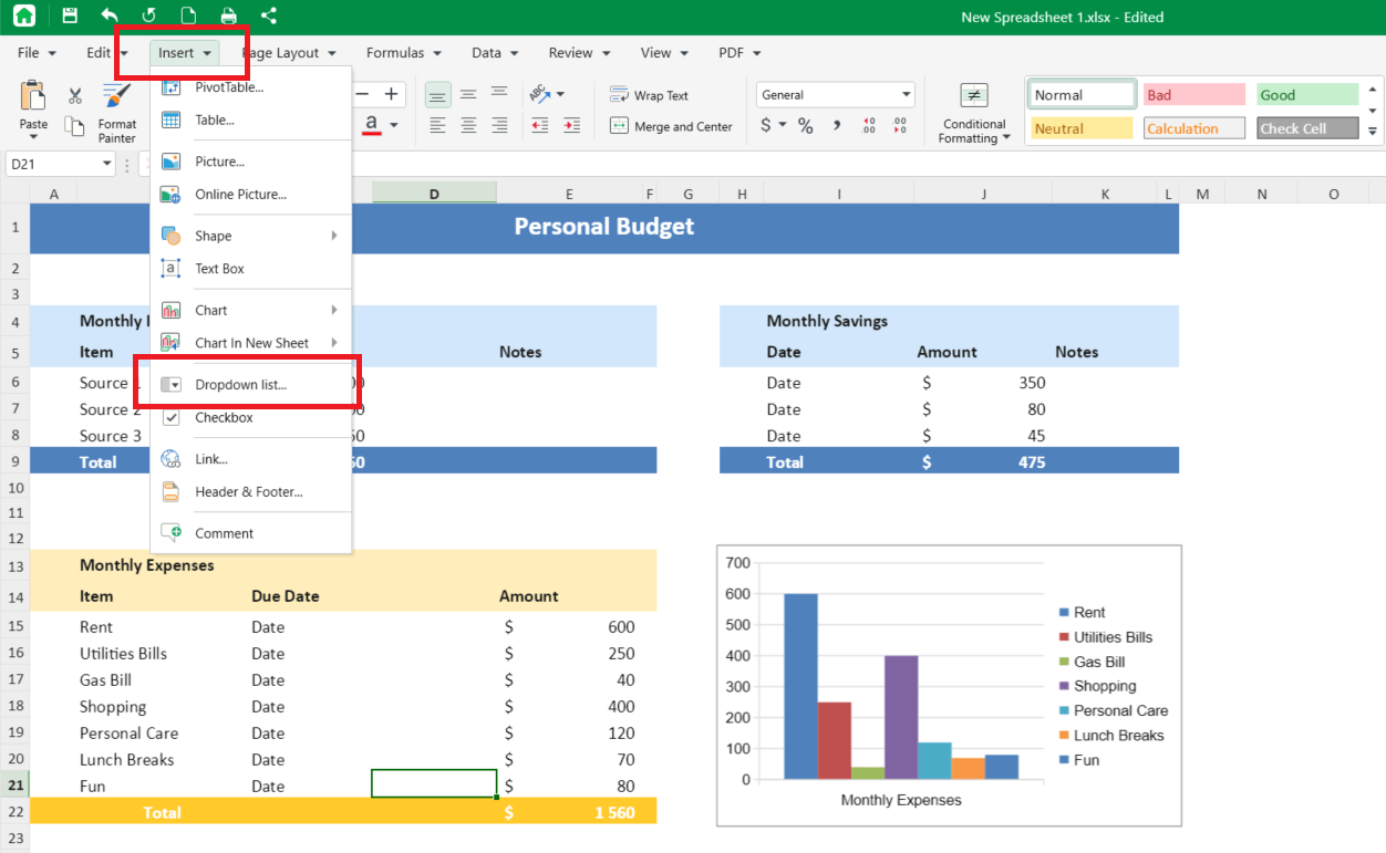
3. The Edit Data Validation pane opens on the right, with Validation Criteria already set to Dropdown.
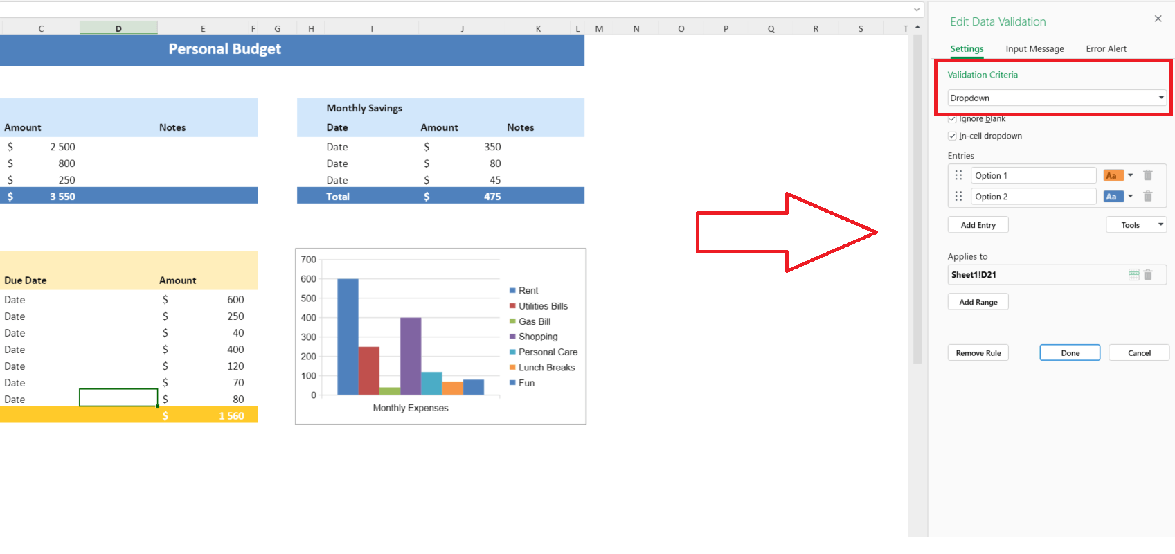
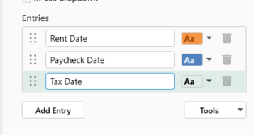
4. Two starter entries, Option 1 and Option 2, appear, each with its own color chip.
5. Rename the entries to match your choices. You can drag entries to reorder them, use the bin icon to remove an option, or click Add Entry to include more.
6. Check Applies to to see the selected range, such as Sheet1!A1. Use Add Range to extend the rule to other cells.
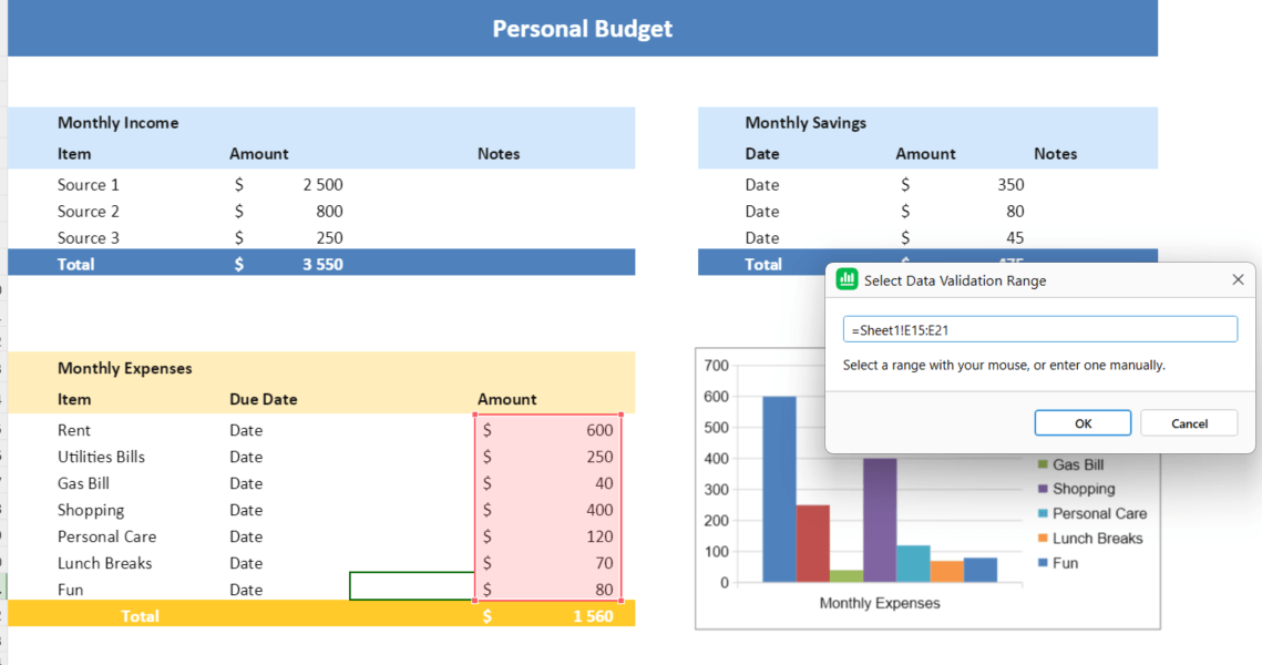
7. Click Done to save the drop-down list.
The Ignore blank and In-cell dropdown options are selected by default. The pane also includes Input Message and Error Alert tabs. You can delete an existing rule using Remove Rule.
Other validation rules are available under Data > Data Validations.
Data Validation is a Premium feature in MobiSheets. With MobiSheets, you get a familiar spreadsheet editing experience if you are looking for an alternative to Microsoft Excel.
To use MobiSheets alongside the other MobiOffice apps, download the suite and choose the plan that suits your needs.
Frequently asked questions
Select the cells where you want the list, then go to Data > Data Validation > Settings. Under Allow, choose List and enter your options in Source, separated by commas, or select a range containing them. Keep In-cell dropdown checked and click OK.
Select a cell with the list and open Data > Data Validation. If you typed the options manually, edit them in Source. If the list references cells, update those values or extend the range. Use Apply these changes to all other cells with the same settings to update matching lists.
Select the cells containing the list, open Data > Data Validation, and click Clear All on the Settings tab. Confirm with OK. Excel removes the validation rule and drop-down arrow but keeps the values already entered in those cells.
The arrow normally appears only when you select a cell containing a drop-down list. If you still can't see it, open Data > Data Validation > Settings and check that In-cell dropdown is selected. Also make sure the cell has a validation rule with Allow set to List.
Yes. You can create a dependent drop-down list using named ranges and the INDIRECT function. Name the source ranges to match the options in the first list, then use a formula such as =INDIRECT(A2) in the second list's Source field to display the corresponding options.
In Excel, you can use conditional formatting to change a cell's appearance based on its selected value. This colors the cell rather than individual entries in the traditional Data Validation list. In MobiSheets, each entry has its own color chip in the Edit Data Validation pane.
Final thoughts
Creating a drop-down list in Excel helps you keep entries consistent and reduce manual typing. For short lists, entering options directly into Data Validation is usually enough. For frequently changing data, a cell range or Excel Table makes updates easier.
You can also use dependent lists when one selection should determine the next. And if your needs change, you can edit or remove the validation rule without starting over.
For another way to manage spreadsheet lists, try MobiSheets as part of the MobiOffice suite.