This article was updated on Feb 18, 2026
You can remove duplicates in Excel by using built-in tools like Remove Duplicates, formulas such as UNIQUE, or conditional formatting to identify repeated values before deleting them. Duplicate data is one of the most common causes of reporting errors, broken formulas, and misleading insights, especially in large or frequently updated spreadsheets.
Knowing how to remove duplicates in Excel is essential for maintaining clean, reliable data. In this guide, you’ll learn how to troubleshoot duplicates that refuse to disappear. We’ll also cover how to handle duplicates in MobiSheets and Google Sheets for faster, more controlled data cleanup.
What does “duplicate data” mean in Excel?
In Excel, duplicate data refers to values or records that appear more than once within a selected range, column, or row set.
Excel considers data duplicates when:
Cell values are identical
Entire rows contain the same combination of values
Data matches exactly across multiple selected columns
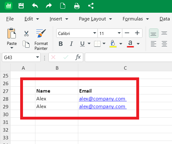
Example: 
This is an exact duplicate row.
However, Excel may not treat the following as duplicates:
Text with extra spaces
Different capitalization (depending on method used)
Values generated by formulas that look the same but evaluate differently
Understanding how Excel defines duplicates is critical before deleting anything.
Why delete duplicates from Excel?
Removing duplicates is important to ensure accuracy in your documents and help decision-making.
Key reasons to remove duplicates in Excel:
Accurate reporting: Duplicate rows inflate totals, averages, and KPIs
Reliable formulas: VLOOKUP, XLOOKUP, and COUNTIF break when duplicates exist
Clean pivot tables: Duplicates distort summaries and groupings
Better automation: Power Query, macros, and workflows rely on clean data
Smarter decisions: Duplicate data leads to false insights and poor business calls
For analysts and operations teams, duplicate cleanup is a foundational step, so it should always be on the agenda.
How to remove duplicates in Excel using the UNIQUE function
Probably the simplest way to remove all duplicates from your spreadsheet is the UNIQUE function as it will scan your range and leave you with just the unique values. The coolest thing about this method is that it will work seamlessly on any spreadsheet software, be it MobiSheets or Google Sheets.
To get this method to work you should:
Select an empty column of your spreadsheet.
Type in the UNIQUE function with your cell range. It should look like this “=UNIQUE(A2:C14)“. You can customize your cell range to your needs.
Hit Enter.
Your unique values will pop up in the empty column.
How to find duplicates in Excel without removing them
If you want visibility before deleting anything, Excel lets you identify duplicates without removing them – here is how.
Use conditional formatting to highlight duplicates:
Select the column or data range
Go to Home → Conditional Formatting
Choose Highlight Cells Rules → Duplicate Values
Pick a formatting style and click OK
Excel instantly highlights all duplicate values, making it easy to review patterns or errors before cleanup.
This method is ideal when you need to:
Audit data quality
Investigate recurring entries
Share findings with stakeholders
How to remove duplicates in Excel (step-by-step)
Excel offers several ways to delete duplicates, depending on whether you want to keep one instance or remove them entirely.
Remove duplicates using the built-in tool:
Select any cell in your dataset
Go to Data → Remove Duplicates
Choose which columns to evaluate
Click OK
Excel removes duplicate rows and keeps the first occurrence by default.
Tip: This action permanently deletes data. Always back up your file or work on a copy.
How to remove duplicates in Excel using a formula
If you want to remove duplicates but keep the first instance, formulas are safer and more flexible.
Use the UNIQUE function:
=UNIQUE(A2:C100)
This creates a new list containing only unique rows, without altering your original data.
Use this approach when you're dealing with:
Large datasets
Dynamic reports
Non-destructive cleanup
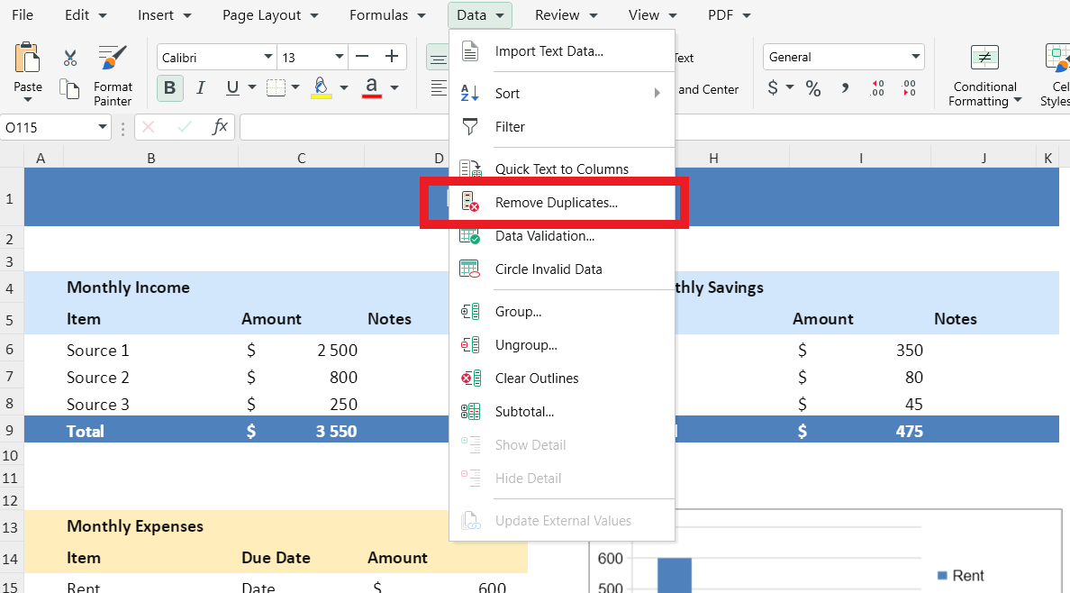
How to remove duplicates from MobiSheets
MobiSheets provides a fast, flexible way to remove duplicates without complex formulas.
Steps:
Select your data range
Click Data → Remove Duplicates

Choose the columns to evaluate.
Confirm headers if applicable.
Click OK
Unlike Excel, MobiSheets gives you more control over how duplicates are detected, making it ideal for business datasets.
Try MobiSheets for faster, safer, and more intuitive duplicate management across all your spreadsheets.
How to remove duplicates from Google Sheets
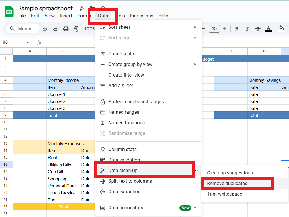
In Google Sheets (web version only):
Select your data range
Click Data → Data cleanup → Remove duplicates

Choose columns and confirm
Click Remove duplicates
You can also use:
=UNIQUE(A:A)
to generate a duplicate-free list without deleting original data.
How to remove duplicates in Excel across multiple columns
To remove duplicates based on multiple columns:
Select the entire dataset
Go to Data → Remove Duplicates
Check all columns that define uniqueness
Click OK
Excel now treats each row as a combined record, removing only exact matches across all selected columns.
How to remove duplicate rows in Excel
Duplicate rows occur when every column value matches another row.
The fastest method:
Select the dataset
Use Remove Duplicates
Select all columns
This ensures only fully identical rows are removed.
Best practices for removing Excel duplicates
To avoid mistakes and loss of important data:
Always work on a copy of your file
Highlight duplicates before deleting
Use formulas for non-destructive cleanup
Clean spaces and formatting before removal
Validate results with counts or pivot tables
For large files, dedicated spreadsheet tools like MobiSheets provide better performance and control.
What to do if your duplicates are still there
If duplicates remain after removal, check for:
Extra spaces or hidden characters
Case-sensitive differences
Formula-generated values
Merged cells
Different data types (text vs numbers)
Use:
=TRIM()
and
=CLEAN()
to normalize data before retrying.
Frequently asked questions
Can I remove duplicates in Excel without deleting the original data?
Yes. Use the UNIQUE function to generate a duplicate-free list while keeping your original dataset intact.
How do I remove duplicates across multiple columns?
Use Data → Remove Duplicates and select all relevant columns to define row uniqueness.
Why does Excel still show duplicates after I remove them?
Hidden spaces, formatting differences, or formulas often cause Excel to treat values as unique.
What’s the safest way to clean duplicates in large Excel files?
Create a backup and use formulas or tools like MobiSheets, which offer better performance and preview options.
How to remove duplicates but keep the first instance in Excel using a formula?
Use:
=UNIQUE(range)
This keeps the first occurrence and removes all subsequent duplicates.
Final thoughts
Duplicate data quietly sabotages spreadsheets. Once you know how to remove duplicates in Excel, you unlock cleaner reports, accurate formulas, and trustworthy insights.
Whether you’re cleaning a customer list or preparing a business report, using the right method matters.


