How to Use Alternate Rows in Excel

Your Excel spreadsheet has to appear professional and organized, but manually shading each row can be time-consuming.

There are quicker ways to give your data a polished look.

How to shade alternate rows in Excel

The two methods below will help you apply alternating colors with minimal effort.

1. Shade alternate rows with Excel’s table style

1. Click any cell within the range of data you want to format.

2. Go to "Insert" and select "Table."

3. Click "OK."

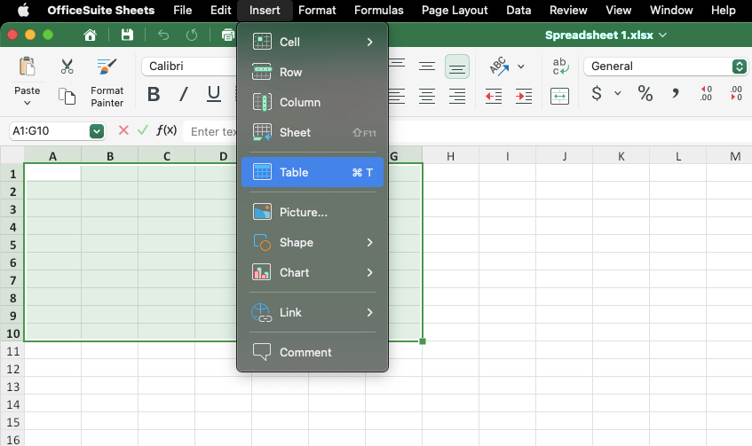
Alternatively, you could:

1. Select the data you want to format. You can either click and drag your mouse across the data or use "Command" (Mac) or "Control" (Windows).

2. Then go to "Home" > "Format as Table."

3. Confirm the cell range and select "OK."

2. Conditional Formatting for alternating rows

If you prefer not to convert your data via table style, use Conditional Formatting.

1. Highlight the cells you want to format.

2. Go to "Home" > "Conditional Formatting".

3. Select "New Rule."

4. Under "Select a Rule Type" > "Use a formula to determine which cells to format."

5. To shade even-numbered rows:

=MOD(ROW(),2)=0

6.To shade odd rows:

=MOD(ROW(),2)=1

7. Click "Format," select a fill color from the "Fill" tab, and click "OK."

You can always edit or remove Conditional Formatting: "Home" > "Conditional Formatting" > "Manage Rules."

How to choose your own colors for table style

So, you've chosen to format your data with tables, but you want to go beyond. Excel offers a variety of preset table styles, which you can easily customize.

1. Format your data as a table.

2. In “Table Design”, browse the "Table Styles" and select a style, under the "Light," "Medium," or "Dark" categories.

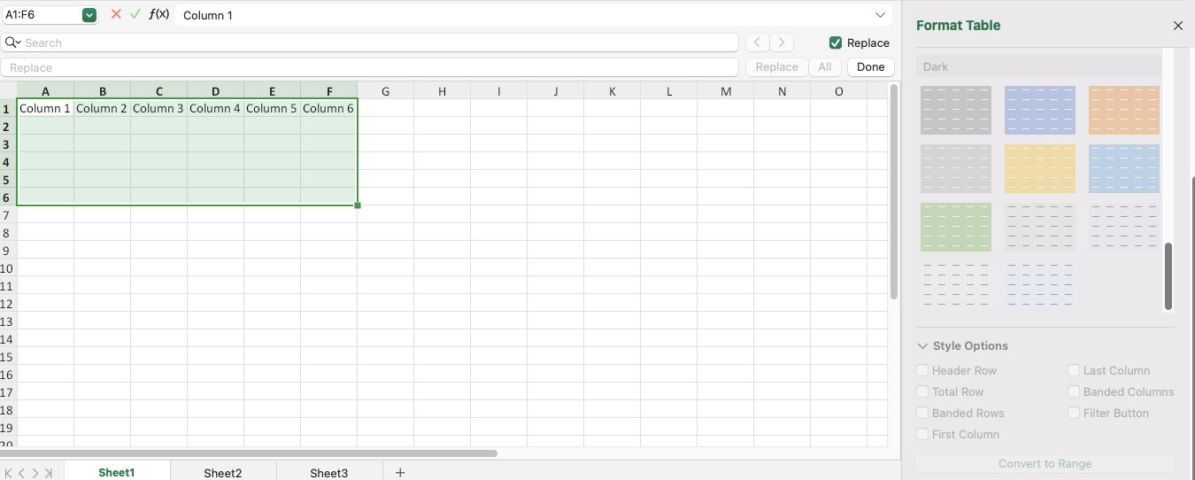
If Excel's preset styles don’t meet your needs, create a custom table style.

1. Go to "Table Design" > "New Table Style".

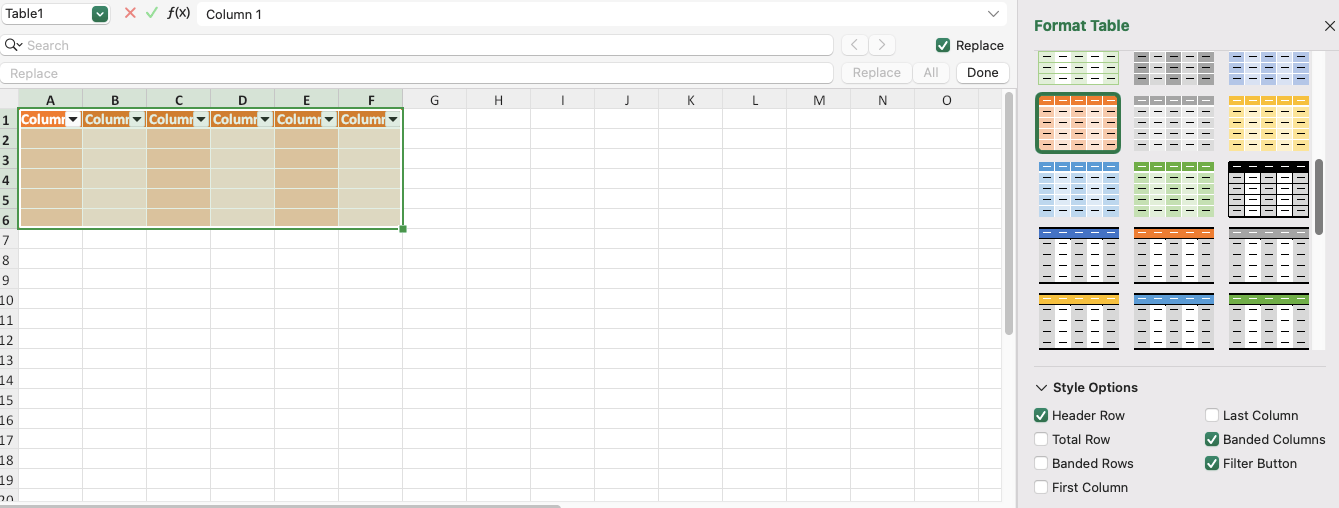
2. Modify elements like the banded rows and headers.

3. Change the shading of specific columns by unchecking the "Banded Rows" box and checking "Banded Columns" in the "Table Style Options".

How to do alternate row shading for different number of rows in every zebra line

What if you want to create an even more unique pattern? Use Conditional Formatting:

1. Go to "Home" > "Conditional Formatting" > "New Rule" > “Use a formula to determine which cells to format”.

2. To shade two rows on and two rows off:

   =MOD(ROW(),4)<2

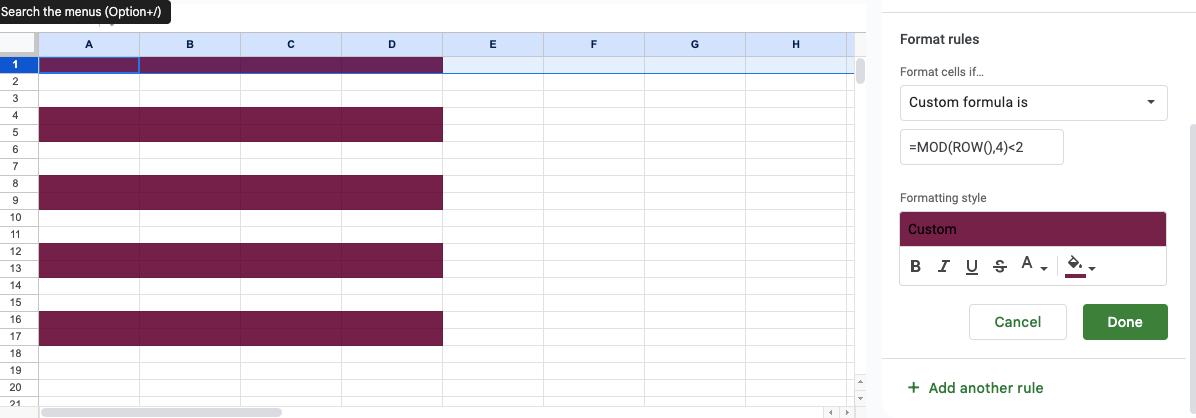
4. To shade three rows shaded and leave one unshaded:

=MOD(ROW(),4)<>1

5. To shade one row and leave two unshaded:

=MOD(ROW(),3)=1

6. Next, click "Format" >"Fill" to customize your design.

7. Click "OK."

If you need to adjust the shading range, go to "Manage Rules," under Conditional Formatting, and edit the "Applies to" field.

How to highlight rows with 3 different colors

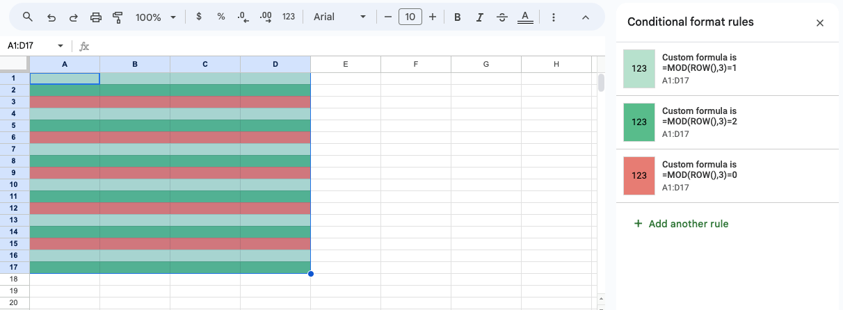
Take your creativity to the next level by using three different colors to shade alternating rows with Conditional Formatting:

1. From Conditional Formatting, select "Use a formula to determine which cells to format".

2. In the "New Formatting Rule", enter:

   =MOD(ROW(),3)=1 (for the first color)

   =MOD(ROW(),3)=2 (for the second color)

   =MOD(ROW(),3)=0 (for the third color)

3. For each formula, click "Format" > "Fill" to select a color for each rule.

How to alternate row colors based on introduced value

Use Conditional Formatting, if you want your rows to change color based on specific values.

1. From Conditional Formatting > "New Rule" > “Format only cells that contain”.

2. Define your conditions based on a value or text criteria.

   • To change the row color for values greater than 10:

     "Cell Value > 10"

To alternate colors for rows with the word "False":

A1="False"

3. Click "Format" > "Fill" to select a color that corresponds to each rule.

4. Click "OK".

How to delete alternate rows in Excel

There are instances where you'd quickly want to delete your alternating rows.

Manually deleting alternate rows

The manual method is best used for smaller data sets.

1. Manually select the first row you want to delete.

2. Right-click one of the selected rows and choose "Delete".

Deleting with the MOD formula

1. Insert a new column next to your data and label it "Helper."

2. In the first cell of the "Helper" column, enter:

=MOD(ROW(),2)

3. Drag the formula down to apply to all rows.

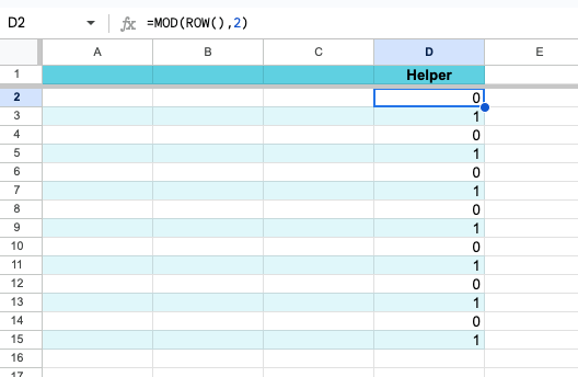
4. Select the "Helper" column and under "Data", choose "Filter" to show only the rows you want to delete.

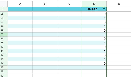
6. Once the rows are filtered, select them, right-click, and choose "Delete".

Using VBA (Visual Basic for Applications)

For larger datasets, VBA can automate the process.

1. Press "Alt" + "F11" to open the VBA editor.

2. Go to "Insert" > "Module."

3. Copy and paste the code into the module window to delete even-numbered rows:

   vba

   Copy code

   Sub DeleteAlternateColumns()

   Dim i As Long

   For i = Columns.Count To 1 Step -1

   If i Mod 2 = 0 Then

   Columns(i).Delete

   End If

   Next i

   End Sub

4. To delete odd rows, use:

   Sub DeleteOddAlternatingRows()

   Dim i As Long

   For i = 1 To Cells(Rows.Count, 1).End(xlUp).Row Step 2

   Rows(i).Delete

   Next i

   End Sub

5. Close the VBA editor.

6. Press "Alt" + "F8" >"DeleteAlternateRows" > "Run."

Filtering to delete alternate rows

1. Select the data range > "Sort & Filter" > "Filter."

2. Click the filter drop-down menu in the column where you want to filter.

3. Choose "Filter by Color", then select the color of the rows you want to delete.

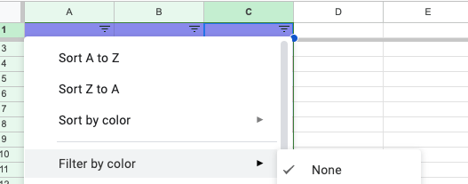
4. Select the visible rows, right-click, and choose "Delete Rows."

5. Remove the filter to reveal the remaining rows.

How to copy and paste alternate rows in Excel

Transfer your data from alternate rows to another Excel worksheet or workbook.

Manual copy-paste

1. Select the first row you want to copy.

2. Hold down the "Ctrl" (or "Cmd") key, and then click each additional row you want to select.

3. Right-click on any selected row and choose "Copy."

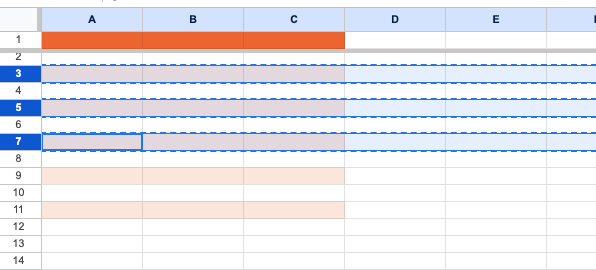
4. Navigate to where you want to move the rows, right-click, and "Paste."

Using formulas to select alternate rows

For larger datasets, use formulas to make the process much more efficient.

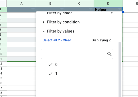
Once again, you'd need to create a "Helper" column to the side of your data. Within its first cell enter and copy down the =MOD(ROW(), 2) formula.

Use the "Sort & Filter" tool to filter by 1 or 0. Select the filtered rows, then copy and paste them into the desired location.

Using VBA macros

If you frequently need to copy and paste alternate rows in large datasets, a macro can automate the process:

1. After you've opened the editor, go to "Insert" > "Module" and paste the following code:

   Sub CopyAlternateRows()

   Dim ws As Worksheet

   Set ws = ActiveSheet

   Dim rng As Range

   Dim i As Long

   Dim copyRange As Range

   For i = 1 To ws.Cells(Rows.Count, 1).End(xlUp).Row Step 2

   If copyRange Is Nothing Then

   Set copyRange = ws.Rows(i)

   Else

   Set copyRange = Union(copyRange, ws.Rows(i))

   End If

   Next i

   copyRange.Copy

   Sheets("Sheet2").Range("A1").PasteSpecial xlPasteValues ' Change Sheet2 to your destination sheet

   End Sub

2. Run the macro by pressing "Alt" + "F8," selecting "CopyAlternateRows," and "Run".

How to select every alternate row in Excel

Find out how to apply bulk formatting to alternate rows by filters, the "Go To Special," and VBA macros.

Filter method

Filtering comes in handy when you want to use alternate rows for calculations.

1. Apply alternate row colors to your table (using "Banded rows").

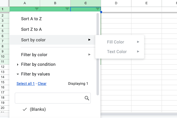
2. Select the table and click "Sort & Filter".

3. From the "Filter" menu, select "By color," then choose the color of the rows you want to highlight.

4. Manually select the rows you want.

Formula and filter method

You can use a helper column and formulas to select odd or even rows.

1. In an empty column, use one of these formulas:

   • For odd rows: =ISODD(ROW())

   • For even rows: =ISEVEN(ROW())

2. Drag and drop it to all columns that follow.

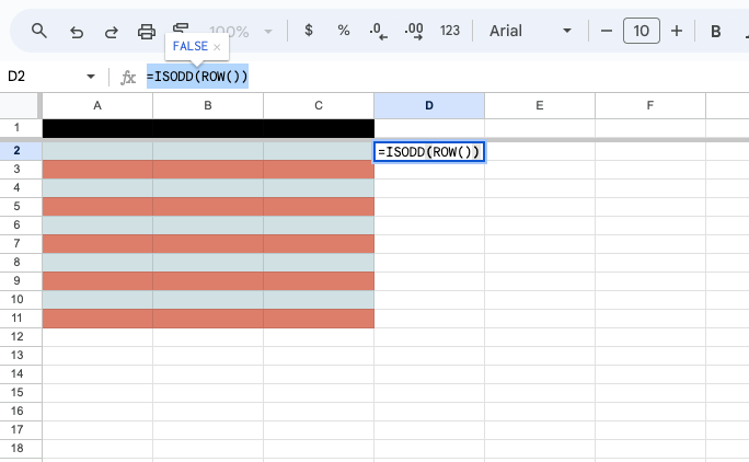
3. Select the table, go to "Data", and click "Filter".

4. Click the filter drop-down and uncheck "TRUE" or "FALSE".

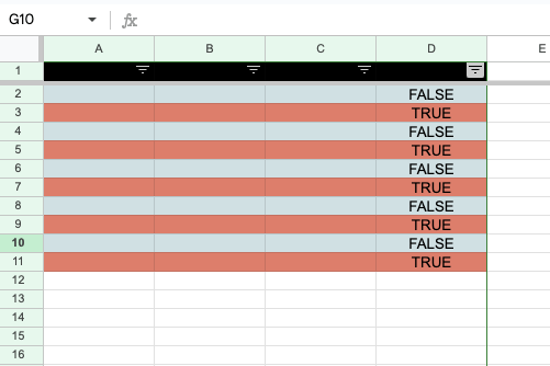
5. Select the filtered rows by dragging or using the "Shift" key.

6. Apply the formatting to the selected rows.

"Go To Special" command method

The "Go To Special" command allows you to select visible rows after applying filters.

1. Go to the "Home" tab and click "Find & Select" > "Go To Special."

2. In the dialog box, choose "Visible Cells only".

3. After selecting, you can delete or modify the selected rows.

VBA Macros to select alternate rows

Select odd rows in VBA:

vba

Copy code

Sub SelectOddRows()

Dim selectedRange As Range

Dim i As Integer

Dim newRange As Range

Set selectedRange = Selection

For i = 1 To selectedRange.Rows.Count Step 2

If newRange Is Nothing Then

Set newRange = selectedRange.Rows(i)

Else

Set newRange = Union(newRange, selectedRange.Rows(i))

End If

Next i

If Not newRange Is Nothing Then newRange.Select

End Sub

Select even rows in VBA:

vba

Copy code

Sub SelectEvenRows()

Dim selectedRange As Range

Dim i As Integer

Dim newRange As Range

Set selectedRange = Selection

For i = 2 To selectedRange.Rows.Count Step 2

If newRange Is Nothing Then

Set newRange = selectedRange.Rows(i)

Else

Set newRange = Union(newRange, selectedRange.Rows(i))

End If

Next i

If Not newRange Is Nothing Then newRange.Select

End Sub

1. Copy and paste one of the above macros into a new module.

2. Press "Alt" + "F8", select your macro (either "SelectOddRows" or "SelectEvenRows"), and "Run."

Final thoughts

To shade alternate rows in Excel, you can use two main methods. The table style method is quick and involves formatting your data as a table, while conditional formatting allows for more customization using formulas like =MOD(ROW(),2)=0 to shade even rows.

Though Excel provides several ways to format alternate rows, if you're looking for a simpler or more user-friendly option, why not try MobiSheets?

MobiSheets offers a more intuitive approach, turning tasks like alternate row shading (or removing duplicates) into a piece of cake.