Does the order of nested IF functions matter?

Yes, the order of nested IF functions is crucial. Excel evaluates each condition in the order it appears, and as soon as one condition is TRUE, the formula stops and returns the corresponding result.You should order your conditions logically – typically from most specific to least specific – is important.

How can I handle errors in my IF formulas?

Errors can occur in IF formulas due to issues like division by zero or referencing invalid data. To manage these gracefully, wrap your IF formula with the IFERROR function.

What Alternatives Are There to IF in Excel? 12 Solutions for Nested IF

Home Blog Tutorials

What Alternatives Are There to IF in Excel?

RMReny Mihaylova

Feb 4, 2025

How do you usually handle decision-making in your professional and everyday Excel worksheets?

For most, the answer is simple: the trusty IF formula. As one of the most popular (and often misused) Excel functions, IF allows you to evaluate data against a single condition.

But what happens when your data requires more than one condition?

Enter the nested IF formula, which enables you to test multiple conditions in a single cell.

While powerful, nested IFs can quickly become confusing and difficult to manage as their complexity grows.

Thankfully, Excel offers a range of alternative formulas that can simplify your work.

In this guide, we’ll explore the mechanics of nested IF functions and introduce you to smarter ways to manage multiple conditions.

What does the IF function do in Excel?

The IF function is a tool for logical comparisons, enabling you to automate responses to varying conditions in your data.

Think of it as a decision-making tool: =IF(Something is True, then do something, otherwise do something else)

=IF(C2="Yes", 1, 2) means: If the value in cell C2 is "Yes," the formula returns 1; otherwise, it returns 2.

You can use the IF function for:

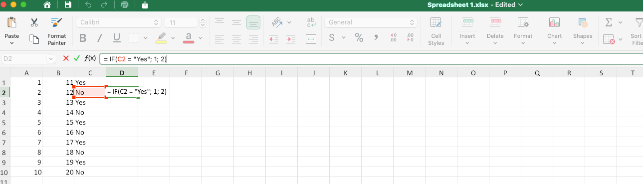
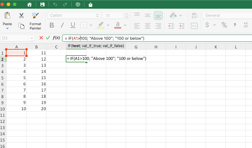
Numeric comparison

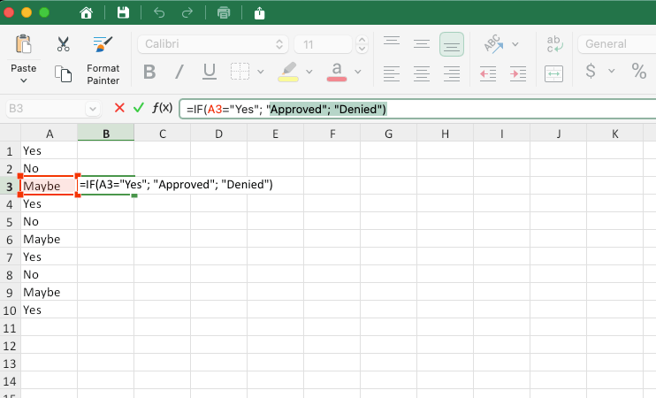
The formula checks whether the value is greater than 100.

Text comparison

The formula returns "Approved" if A3 contains "Yes".

Calculations based on condition

This formula applies a 10% rate if the value is 50 or more; otherwise, it applies a 5% rate.

Why you might want to avoid using the IF formula?

You’d use IF for simple conditions like "Yes"/"No" or "Pass"/"Fail." Once you start layering multiple conditions, things can quickly spiral out of control, as:

A single mistake in your logic or syntax can produce wrong results, especially in large datasets.
Deciphering someone else’s long logic chain wastes time and increases the chances of new errors.
Manually entering conditions and values opens the door to typos and inconsistencies.

Check out the two examples below to see why long formulas can get messy:

Example 1: Discount Tiers

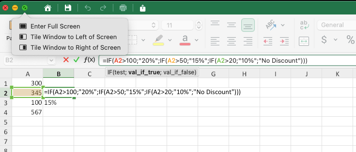
Imagine you’re setting discounts based on order size.

If you decide to offer a new discount for orders over 200, you’ll need to rework the formula.

Forgetting to adjust the order of conditions could easily lead to incorrect outputs, like a customer qualifying for only 15% instead of 20%.

Example 2: Employee Bonuses

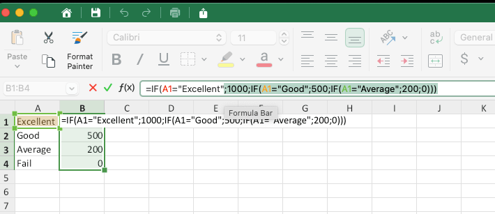
You calculate bonuses based on performance ratings.

What happens if your HR team introduces new performance categories like "Outstanding" or "Needs Improvement"?

Each change requires carefully rechecking the formula, and a small oversight could mean bonuses are calculated incorrectly.

What is a nested IF function?

Sometimes your data requires more than a simple "TRUE"/"FALSE" test.

Nested IF functions allow you to include multiple IF statements, allowing you to test several conditions and return different outcomes based on each.

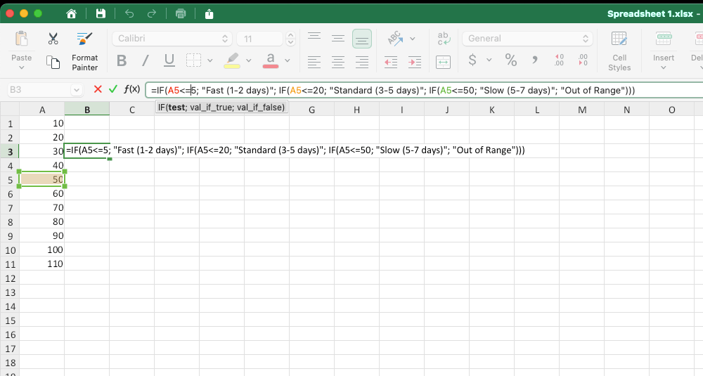
For example, imagine you’re running a delivery service and want to categorize delivery times based on the distance in kilometers.

Here's how the complete formula would look like: =IF(A5<=5, "Fast (1-2 days)", IF(A5<=20, "Standard (3-5 days)", IF(A5<=50, "Slow (5-7 days)", "Out of Range")))

How to build nested IF statements

Here are our top three tips for managing your nested IF statements:

1. Match your parentheses carefully

The nested IF formula requires careful pairing of parentheses, as misplaced or unmatched parentheses will cause errors.

2. Treat text and numbers correctly

Always enclose text values in double quotes, but leave numbers without quotes.

Correct: 50 has no quotes.

Incorrect: the number is in quotes.

3. Use line breaks and spacing

Use line breaks (press "Alt" + "Enter") or spaces to make longer IF formulas easier to read.

What can you use instead of a nested IF function?

Nested IF functions come with significant downsides as their complexity grows.

Long, intricate formulas quickly become hard to understand, debug, and maintain, especially for others working on the same spreadsheet.

Luckily, Excel offers several alternatives to replace nested functions. Here are some of the best options, along with examples to help you simplify your workbooks:

VLOOKUP for hierarchical values

When working with scales or continuous numerical ranges, a VLOOKUP formula with an approximate match can replace the lengthy nested IF function.

Use this formula to look up values that fall between set thresholds.

Scenario: discount based on purchase amount

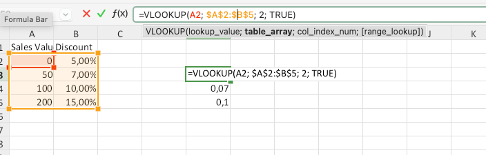
Create a reference table and use this formula: =VLOOKUP(A2, $A$2:$B$5, 2, TRUE)

"A2" contains the sales value. The formula looks up the value in the range $A$2:$B$5 and retrieves the corresponding discount from column 2.

CHOOSE & MATCH for fixed sets

When dealing with predefined values that map directly to outcomes, the CHOOSE and MATCH combination can streamline your formulas.

Scenario: employee ratings based on performance

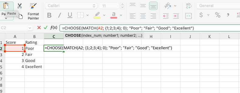
Here’s the formula: =CHOOSE(MATCH(A2, {1,2,3,4}, 0), "Poor", "Fair", "Good", "Excellent")

MATCH(A2, {1,2,3,4}, 0) finds the position of the score in the list {1,2,3,4}.

CHOOSE uses this position to return the corresponding rating.

SWITCH function for single expressions

The SWITCH function is perfect for evaluating one expression against multiple possible values.

Scenario: grading system by letter grade

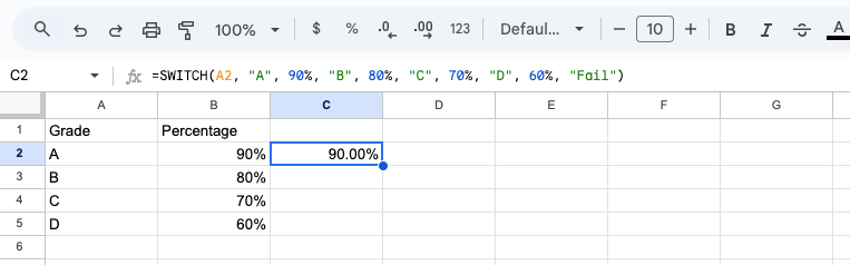
Use the SWITCH function: =SWITCH(A2, "A", 90%, "B", 80%, "C", 70%, "D", 60%, "Fail")

SWITCH evaluates the value in "A2" against the list of possible grades and returns the corresponding percentage.

IFS function for multiple logical tests

The IFS function simplifies multiple conditions into a clean and readable formula, evaluating each condition sequentially, and returning the value for the first "TRUE" condition.

Scenario: delivery times based on distance
Let’s revisit the delivery service example!

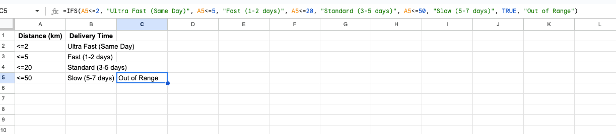
Use this formula: =IFS(D5<=2, "Ultra Fast (Same Day)", D5<=5, "Fast (1-2 days)", D5<=20, "Standard (3-5 days)", D5<=50, "Slow (5-7 days)", TRUE, "Out of Range")

Each condition (D5<=2, D5<=5, etc.) is evaluated in order, where either the corresponding value or "Out of Range" is returned.

Boolean logic for numerical scenarios

Boolean logic leverages Excel’s internal handling of "TRUE" as 1 and "FALSE" as 0 to simplify formulas and works best with numerical values.

Scenario: Currency conversion

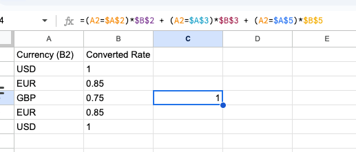
If you’re converting currencies, use: =(A2=$A$2)*$B$2 + (A2=$A$3)*$B$3 + (A2=$A$5)*$B$5

Each logical test (A2=$A$2) evaluates to "TRUE" (1) or "FALSE" (0).

Multiplying the result by the corresponding exchange rate (e.g., $B$3) ensures only the correct rate is added to the total.

REPT for text-based scenarios

The REPT function is an unconventional yet effective way to return specific values based on conditions, especially for text.

Scenario: Labeling categories

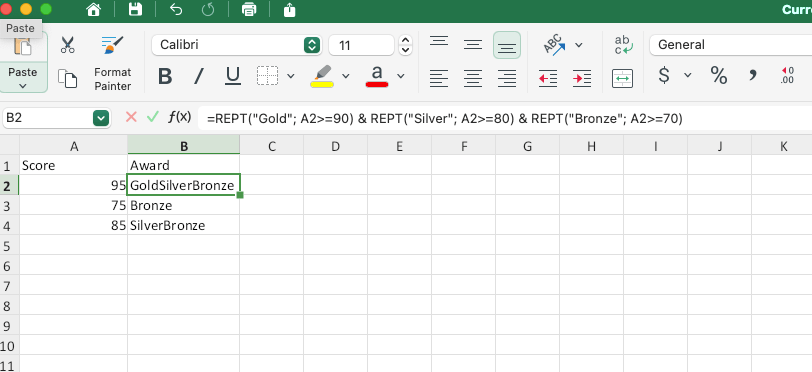
For categories like "Bronze," "Silver," and "Gold," use: =REPT("Gold", A2>=90) & REPT("Silver", A2>=80) & REPT("Bronze", A2>=70)

Here's how it works REPT function returns all the listed criteria.

When dealing with large datasets or summary calculations, consider using pivot tables. They allow you to group, filter, and summarize data without the need for complex formulas.

How do you use an array formula?

An array formula allows you to perform multiple calculations on a range of data simultaneously, either a single result or multiple results.

Often referred to as CSE ("Ctrl"+"Shift"+"Enter") formulas, these formulas require pressing the three-button sequence.

Array formulas are ideal for replacing IF statements when dealing with dynamic ranges or complex criteria, as they allow you to reference entire ranges of data.

These functions are easier to maintain – if conditions change, you only need to update the referenced range.

SUMPRODUCT for conditional calculations

SUMPRODUCT multiplies the matching 1 with the rates and sums the result.

Scenario: Total sales commission based on the region

Use SUMPRODUCT: =SUMPRODUCT(--(A2=$A$2:$A$5),$B$2:$B$5)

--(A2=$A$2:$A$5) creates an array of 1 for the matching region and 0 for others.

$B$2:$B$5 contains the corresponding commission rates.

INDEX function & MATCH for dynamic lookups

Scenario: Tax rate for a given income bracket

Use index match: =INDEX($B$2:$B$4,MATCH(TRUE,A2>=$A$2:$A$4,1))

MATCH(TRUE,A2>=$A$2:$A$4,1) finds the highest bracket that matches the income.

The INDEX function returns the corresponding tax rate based on the position.

FILTER for advanced filtering

The FILTER function dynamically updates when data changes, unlike a static nested IF.

Scenario: Extract all products with sales greater than $10,000

Use FILTER: =FILTER(A2:B4,B2:B4>10000)

FILTER retrieves rows where the sales column (B2:B4) exceeds 10,000.

MAXIFS/MINIFS for conditional extremes

Scenario: Maximum or minimum sales for a specific product

Use MAXIFS to find the highest sales in the "Food" category.

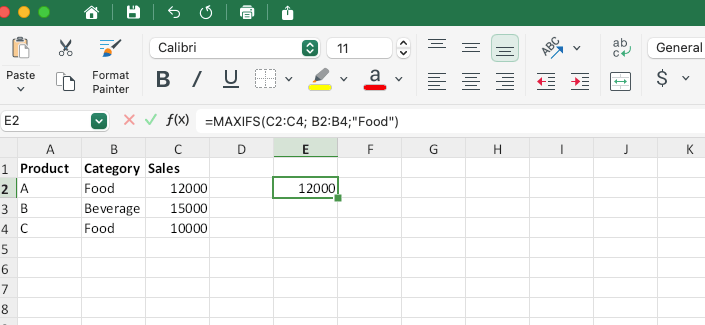
Here's the function: =MAXIFS(C2:C4,B2:B4,"Food")

MAXIFS evaluates the sales in C2:C4 for rows where B2:B4 equals "Food" and returns the highest value.

AVERAGEIFS for conditional averages

Scenario: average sales for "Beverage"

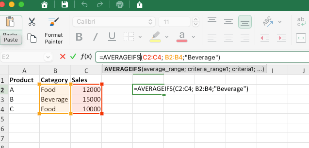
Use the AVERAGEIFS function: =AVERAGEIFS(C2:C4,B2:B4,"Beverage")

AVERAGEIFS averages the sales in C2:C4 for rows where B2:B4 equals "Beverage."

XLOOKUP for exact and approximate matches

Scenario: Look up a product’s price

The XLOOKUP function =XLOOKUP(A2,$B$2:$B$4,$C$2:$C$4,"Not Found")

XLOOKUP searches for A2 in the product list ($B$2:$B$4) and returns the corresponding price from $C$2:$C$4.

While Excel provides numerous functions to streamline data analysis, other platforms (i.e. MobiSheets and Apple's Numbers) also offer robust spreadsheet solutions.

Conclusion

IF and the nested IF functions are powerful tools, but they can quickly become overwhelming as complexity grows.

Thankfully, Excel provides a range of alternatives – such as IFS, VLOOKUP, and array formulas – that simplify logic and make your spreadsheets more efficient.

By using these smarter solutions, you can save time, reduce errors, and enhance your decision-making.

Ready to streamline your workflow? Try MobiSheets today and experience a more intuitive way to manage your data!

Free Download

FAQ

In Excel 2007 and later (including Excel 365), you can nest up to 64 IF functions in a single formula.

While 64 levels provide a lot of flexibility, it’s rarely practical to use that many nested IFs. Long, complex formulas are harder to debug and maintain.

If you find yourself using too many nested IFs, consider switching to alternatives like IFS, VLOOKUP, or SUMPRODUCT for a cleaner, more efficient approach.