
If you’ve ever worked with a big Excel spreadsheet, you probably know this scenario well: you scroll down to row 37, and suddenly you can’t remember what each column was supposed to represent. Their names have moved up and now, you’re just not sure. Was column D the budgeted amount or the actual cost? Without your header rows visible, it’s like navigating a maze blindfolded.
That’s where freezing rows in Excel comes to the rescue. Freezing lets you lock headers, specific rows, or even a combination of rows and columns in place, so you can always see the context of your data, no matter how far you scroll.
In this easy guide, you’ll learn how to freeze the top row, specific rows, and both rows and columns together; how to unfreeze them when you’re done; the most common mistakes to avoid; and why freezing rows is so useful in real-world scenarios.
So, let’s dive in!
Why freezing rows is so useful in Excel
So, why spend time learning this simple feature? Because freezing rows and columns can completely change the way you navigate and interpret your data. It always keeps key information visible, no matter how large or complex your worksheet becomes. When you can always see your headers, categories, or key labels, it’s easier to stay organized and make accurate decisions.
Below, we’ve included a few practical examples of how different users benefit from this super useful habit.
For data analysts
Keeping variables or field names visible while scrolling through thousands of records ensures accuracy and helps spot trends without constantly losing track of what each column represents.
For project managers
Freezing task names while monitoring timelines or deadlines allows you to follow progress effortlessly and keep your schedules aligned.
For teachers and students
In grade books or attendance sheets, keeping student names and assignment titles visible at the same time prevents confusion and helps maintain clear, structured records.
For business users
When reviewing sales reports or comparing performance across regions, it’s easier to match numbers with the correct months or categories when the headers remain visible.
So freezing rows and columns is not just a convenient feature. It provides structure, prevents errors, and helps you work more confidently and efficiently within your data.
How do you freeze the top row in Excel?
Let's go ahead and answer this so common question: how do you freeze the top row in Excel? Common, because in most spreadsheets, the first row contains your headers (titles like “Name”, “Date”, “Amount”) and losing sight of those while scrolling makes analysis almost impossible.
Here’s the quick solution:
1. Open your Excel file.
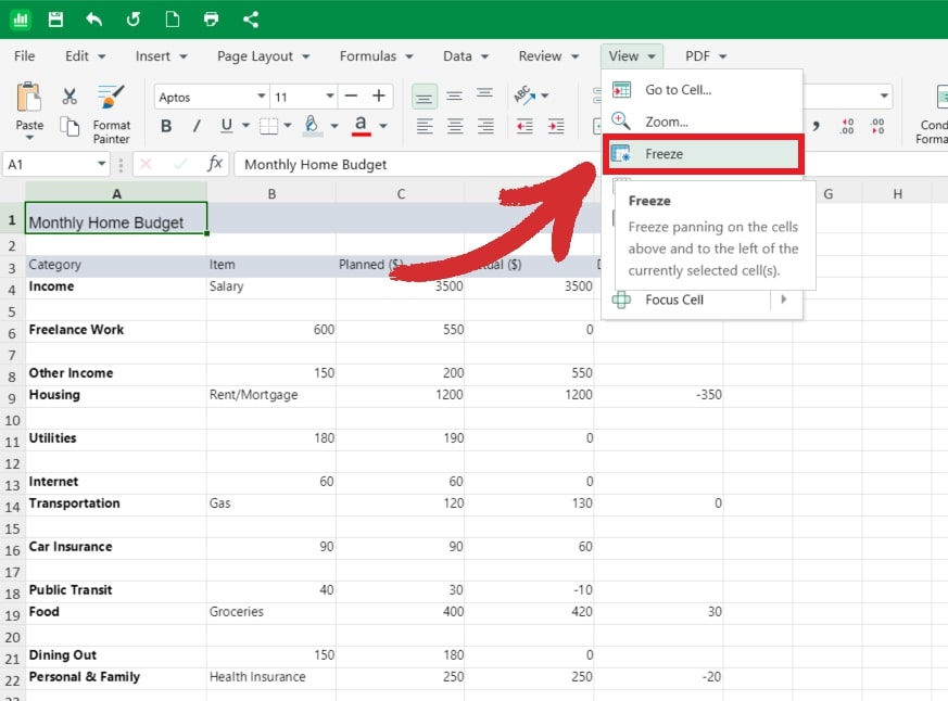
2. Go to the View tab on the Ribbon.
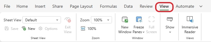
3. In the Window group, click Freeze Panes.
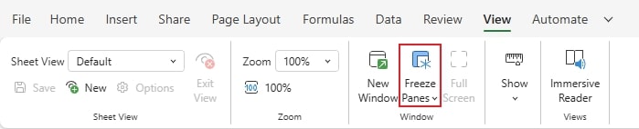
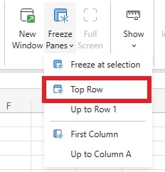
4. Select Top Row.
After you do that, a thin horizontal line will appear just below row 1, showing that the freeze is now active.
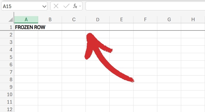
So, if you want to scroll down to row 10, 100, or 54 747, your top row will always remain visible like a header for your spreadsheet.
Of course, this feature is also readily available in MobiSheets – and it’s easier to use than ever. Simply go to View → Freeze and choose the option you need to instantly start making sense of your data.
Note that if your headers are actually on the second row (maybe the first row is just a title), Excel will only freeze the very first row. In that case, you’ll want to use the “Freeze Panes” option to customize what gets locked. Keep reading to find out what these options are.
How to freeze a specific row in Excel (or multiple rows)?
Sometimes, your headers aren’t in row 1. Maybe row 1 is a title, row 2 has some notes, and row 3 is where your actual column headers start. In that case, the question becomes: how to freeze a particular row in Excel?
Here’s what you need to do:
1. Click on the row you want to freeze.
2. Go to View → Freeze Panes.
3. Choose Freeze at selection.

Excel will now lock everything above your selected row. That means you can freeze multiple rows at once by selecting the row right beneath them.
Pro tip: This is especially useful when working with datasets where important details (like categories or sub-headers) stretch across more than one row.
Make sense of your numbers with MobiSheets for Windows, macOS, or mobile. Track budgets, manage reports, and visualize data in an easy-to-use app.
How to freeze a row and column in Excel?
If you need to freeze your first column, simply click “First Column” to lock it neatly in place.
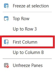
A vertical line will then appear indicating that your column is frozen, like so:

But what if you need both headers at the top and a column on the left locked in place? For instance, maybe your first column contains shopping item names or a monthly budget expense, and you don’t want those to disappear as you scroll sideways.
Here’s how to freeze a row and column in Excel simultaneously:
1. Click next to the row and column you want to freeze, e.g. click on B2 to freeze row 1 and column A.
2. Go to View → Freeze Panes.
3. Choose Freeze at selection.
Now, both the selected row and column will stay visible no matter how far you scroll horizontally or vertically.
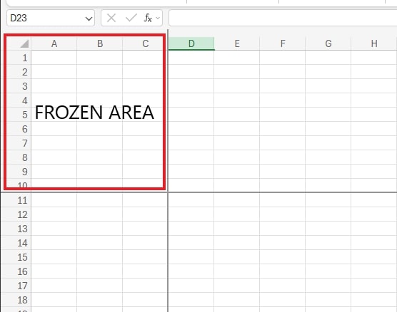
Pro tip: You can use this to lock multiple rows and columns. For instance, if you click on D11, you’ll freeze both rows 1-10 and columns A-C, like so:
How to unfreeze rows or columns in Excel?
Sometimes, you only need the freeze function temporarily. Maybe you were preparing a report, cleaning up your data, or comparing numbers across a long sheet, and now that you’re done, you want everything to scroll freely again.
Luckily, removing a freeze is just as simple as setting one up.
Here is how you do it:
1. Go back to View → Freeze Panes.
2. Click Unfreeze Panes.
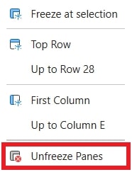
Your worksheet will instantly return to normal scrolling, so you can move up and down the sheet without any locked rows or columns getting in the way.
Pro tip: If you’ve got multiple freezes active, a single click on Unfreeze Panes removes them all.
How do you know if “Freeze Panes” is active?
It’s not always obvious whether a freeze worked, especially when you’re dealing with large datasets that stretch across hundreds of rows or multiple columns. You might think the feature is active, but scrolling down only to see your headers disappear can be confusing.
Here’s how to double-check:
1. Look for the freeze line.
A thin, dark grey line between rows or columns is your visual cue that the freeze is active. It separates the frozen section from the scrollable area of your worksheet.
2. Try scrolling.
Move down or sideways through your data. If your header row or first column stays visible while everything else moves, the freeze is working as intended.
3. Check the menu option.
Go to View → Freeze Panes. If you see Unfreeze Panes instead, that’s another sign your sheet currently has frozen sections.
Bonus tip: If you’re working on a shared or complex file, it can help to quickly toggle the freeze off and on to verify which areas are locked. This ensures everyone looking at the sheet sees the same layout and scrolling behavior.
By using these quick checks, you can confirm that your frozen panes are active – and avoid any confusion when navigating through large spreadsheets.
Need to work with pivot tables instead? Learn all there is to know about one of the most important features found in any spreadsheet software and elevate your workflow.
Common mistakes when freezing rows in Excel
Even though freezing rows or columns in Excel seems straightforward, there are a few common mistakes that can trip you up – especially if you’re working fast or switching between sheets. Understanding these small details will help you avoid confusion and make the feature work exactly as intended.
1. Selecting the wrong row or column
It’s easy to misjudge where to click before applying the freeze. Remember, Excel freezes everything above and to the left of your current selection.
Solution: Always select the row below or the column to the right of what you want to keep visible. For example, to freeze Row 1, click any cell in Row 2 before choosing View → Freeze Panes.
2. Trying to freeze while editing a cell
If your cursor is blinking inside a cell, meaning you’re actively editing it, Excel won’t apply the freeze. The command will simply be ignored.
Solution: To fix this issue, press “Enter” or “Esc” on your keyboard to exit edit mode before using Freeze Panes.
3. Working with protected sheets
When a worksheet is locked or protected, some view and layout options (including Freeze Panes) may be disabled.
Solution: Go to Review → Unprotect Sheet (if you have permission) to temporarily unlock the sheet, apply the freeze, and then protect it again if needed.
4. Forgetting that freezing is sheet-specific
A common surprise for new users: freezing rows or columns applies only to the current sheet. If you switch to another tab, you’ll need to set up the freeze again.
Solution: Each worksheet in a workbook has its own view settings – so repeat the process on every tab where you need frozen headers.
By keeping these simple details in mind, you’ll avoid the most frequent issues and make sure your freezes behave the way you expect, every time.
Frequently asked questions
Can I freeze more than one row or column at a time?
Yes! In Excel, you can freeze multiple rows or columns by selecting the cell just below the last row and to the right of the last column you want frozen, then choosing View → Freeze Panes. This will ensure everything above and to the left of your selection will stay visible while you scroll.
Why can’t I freeze panes in my worksheet?
There are a few reasons this might happen. Make sure you’re not actively editing a cell, because Excel won’t apply the freeze while in edit mode. Also, check if the sheet is protected – some options, including Freeze Panes, are disabled on locked sheets. Finally, remember that freezing applies only to the active sheet, so it won’t carry over to other tabs automatically.
How do I know if my freeze is active?
Look for a thin line between rows or columns – this indicates the frozen section. You can also scroll through your sheet; if the headers or frozen columns remain visible, the freeze is active. Another clue is that the Freeze Panes menu changes to Unfreeze Panes when a freeze is applied.
Can I freeze rows and columns on Excel for the web?
Yes! Excel for web supports freezing rows and columns using the same steps: go to View → Freeze Panes, then choose the appropriate option. The functionality is very similar to the desktop version.
What’s the difference between freezing the top row and using Freeze Panes?
Freezing the top row is a one-click solution that locks only row 1. Freeze Panes gives you more flexibility, allowing you to freeze any combination of rows and columns, which is useful when headers or labels are not in the first row or column.
Can I use the same freeze functionality in MobiSheets?
Absolutely. MobiSheets offers the same freeze panes functionality as Excel. You can lock rows, columns, or both simultaneously, scroll through large datasets with ease, and work across desktop, tablet, or mobile devices.
MobiSheets: An Excel-friendly alternative with Freeze functionality
Freezing rows in Excel is powerful – but what if you want an alternative that’s equally capable, more affordable, and works anywhere? That’s where MobiSheets comes in.
MobiSheets is fully Excel-compatible, so you can open, edit, and save your existing spreadsheets without a hitch. It also supports:
Freeze panes: Lock rows and columns, just like in Excel.
Large table handling: Scroll through big datasets with ease.
Cross-device access: Work on your spreadsheets from desktop, tablet, or phone.
Affordable plans (including a free version!): Perfect for anyone who wants Excel’s power without Excel’s price tag.
If you’ve ever used Excel, MobiSheets will feel instantly familiar – but lighter, smarter, and more flexible.
Try MobiSheets today and see why it’s the perfect tool for innovators who want to get more done on any device.